Duplicate Values

Testing A List For Duplicate Items

The formula below will display the words "Duplicates" or "No Duplicates" indicating whether there are duplicates elements in the list A2:A11.

=IF(MAX(COUNTIF(A2:A11,A2:A11))>1,"Duplicates","No Duplicates")

An alternative formula, one that will work with blank cells in the range, is shown below. Note that the entire formula should be entered in Excel on one line.

=IF(MAX(COUNTIF(INDIRECT("A2:A"&(MAX((A2:A11<>"")*ROW(A2:A11)))),
INDIRECT("A2:A"&(MAX((A2:A11<>"")*ROW(A2:A11))))))>1,"Duplicates","No Duplicates")

Highlighting Duplicate Entries

You can use Excel's Conditional Formatting tool to highlight duplicate entries in a list. All of the examples in this section assume that the data to be tested and highlighted is in the range B2:B11. You should change the cell references to the appropriate values on your worksheet.

This first example will highlight duplicate rows in the range B2:B11. Select the cells that you wish to test and format, B2:B11 in this example. Then, open the Conditional Formatting dialog from the Format menu, change Cell Value Is to Formula Is, enter the formula below, and choose a font or background format to apply to cells that are duplicates.

=COUNTIF($B$2:$B$11,B2)>1

The formula above, when used in Conditional Formatting, will highlight all duplicates. That is, if the value 'abc' occurs twice in the list, both instances of 'abc' will be highlighted. This is shown in the image to the left, in which all occurrences of 'a' and 'g' are higlighted.

You can use the following formula in Conditional Formatting to highlight only the first occurrence of an entry in the list. For example, the first occurrence of 'abc' will be highlighted, but the second and subsequent occurrences of 'abc' will not be highlighted.

=IF(COUNTIF($B$2:$B$11,B2)=1,FALSE,COUNTIF($B$2:B2,B2)=1)

This is shown at the left where only the first occurrences of the duplicate items 'a', 'e', and 'g' are highlighted. The second and subsequent occurrences of these values are not highlighted.

You can also do the reverse of this with Conditional Formatting. Using the formula below in Conditional Formatting will highlight only the second and subsequent occurrences of a value. The first occurrence of the value will not be highlighted.

=IF(COUNTIF($B$2:$B$11,B2)=1,FALSE,NOT(COUNTIF($B$2:B2,B2)=1))

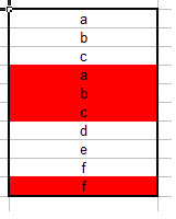
This is shown at the left where only the second occurrences of 'a', 'b', 'c' and 'f' are highlighted. The first occurrences of these items are not highlighted.

Another formula for Conditional Formatting will highlight only the last occurrence of a duplicate element in a list (or the element itself if it occurs only once).

=IF(COUNTIF($B$2:$B$11,B2)=1,TRUE,COUNTIF($B$2:B2,B2)=COUNTIF($B$2:$B$11,B2))

As you can see only the last occurrences of elements 'a', 'b', 'c', and 'f' are highlighted. Element 'd' is highlighted because it occurs only once. The occurrences of 'a', 'b', 'c' and 'f' that occurs before the last occurrence are not highlighted.

We can round out our discussion of highlighting duplicate rows with two additional formula related to distinct items in a list.

The following can be used in Conditional Formatting to highlight elements that occur only once in the range B2:B11.

=COUNTIF($B$2:$B$11,B2)=1

This image illustrates the formula. Elements 'b', 'c', and 'e' are highlighted because they occur only once in the list. Items 'a', 'd' and 'f' are not highlighted because they occur more than one time in the list.

Finally, the following formula can be used in Conditional Formatting to highlight the distinct values in B2:B11. If an element occurs once, it is highlighted. If it occurs more then once, then only the first occurrence is highlighted.

=COUNTIF($B$2:B2,B2)=1

As you can see, only the first or only occurrences of the elements are highlighted. If an element is duplicated, as is 'b', the duplicate elements are not highlighted.

Counting Distinct Entries In A Range

The following formulas will return the number of distinct items in the range B2:B11. Remember, all of these are array formulas.

The following formula is the longest but most flexible. It will properly count a list that contains a mix of numbers, text strings, and blank cells.

=SUM(IF(FREQUENCY(IF(LEN(B2:B11)>0,MATCH(B2:B11,B2:B11,0),""), IF(LEN(B2:B11)>0,MATCH(B2:B11,B2:B11,0),""))>0,1))

If your data does not have any blank entries, you can use the simpler formula below.

=SUM(1/COUNTIF(B2:B11,B2:B11))

If your data has only numeric values or blank cells (no string text entries), you can use the following formula:

=SUM(N(FREQUENCY(B2:B11,B2:B11)>0))